The purpose of this assignment is giving you an intuition about HMMs using RNN. Therefore, you will be developing an HMM by developing RNN using the same building blocks provided in the previous assignment. Briefly, instead of traversing through the states of the HMM trellis, you will be propagating through neural network layers. Since you are already familiar with the feedforward neural networks, you are expected to build sequences of feedforward neural networks for given training data. You will see that why do you need to build sequences of feedforward neural networks in next chapters but, as a spoiler, RNNs are just feedforward neural networks in a loop where each feedforward neural network has two inputs, output of previous neural network t-1 and input element at time t. Key problem you are going to encounter is dynamic input. You are provided with the same dataset as you used for your previous assignment which has a dynamic range of sentence sizes. In order to handle static input size of 4 you need to design your RNN as example code suggests, also you need to modify the get feature function accordingly. RNN with dynamic input has no limitation about the sentence size so you need to figure out how are you going to use your get_feature function and recurring the hidden layer as much as input size so your RNN will be handling a variable size of input in the dataset. As a final note, you are again obliged to report your steps and results using scientific methodology.
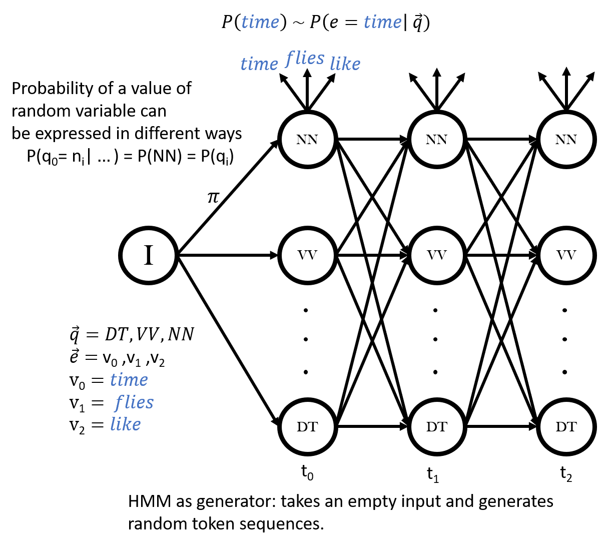
As you have learned in the class, HMMs can be used as generative models where the output sequences are randomly generated following the distribution described by the initial probabilities, transition probabilities, and emission probabilities. Recall that the probability distribution for the random variable q (state) describes how the probabilities over the values n (nodes) are distributed, and the probability distributions for the random variable e (emission) describes how the probabilities over the values v (vocabulary) are distributed. Thinking metaphorically in terms of the dice rolling story, at each time step t, we roll a transition dice weighted by underlying distribution of the random variable qt in order to choose which node n to move to, followed by an emission dice weighted by the underlying distribution of the random variable et in order to choose which vocabulary item v to emit.
Consider the above trellis representing an HMM unrolled in time. In the
dice rolling generative story, first a transition dice is rolled to draw
the value of q0 following a distribution over POS
tags where the value of the drawn hidden state is ni
with the transition probability π = P(q0 = ni).
For the sake of concreteness, in above example let's suppose the dice roll
results in NN, which means that ni is NN. The next
step is to roll an emission dice weighted by the probability P(e0
= vi) in order to draw the value of e0 which will be
the first generated token of the sequence, v0 .
Again for the sake of concreteness, in above example, let's suppose the
dice roll results in time
which means that v0 is
time
. This generative process repeats for each time step t
until the end of the trellis where all emissions are e0,
e1 and, e2 with values time
,
flies
, and like
respectively.
Now as a step toward RNNs, the question is: can we instead somehow use a feedforward network in some analogous way to generate sequences? And if we can, how similar and/or interchangeable are RNNs and HMMs? To answer such questions we first need a basic understanding of feedforward neural networks. Luckily you are already familiar with them as you now have a considerable amount of experience from your previous assignment.
To help us stay oriented, here are the symbol names for random variables and values for HMMs. We're going to ask if we can come up with analogous entities in a feedforward network architecture.
| HMM symbols |
RNN symbols |
|
| Random Variable (R.V.) For the States |
qt | |
| State values | ni | |
| Random Variable (R.V.) For the emissions |
et | |
| Emission values | vi |
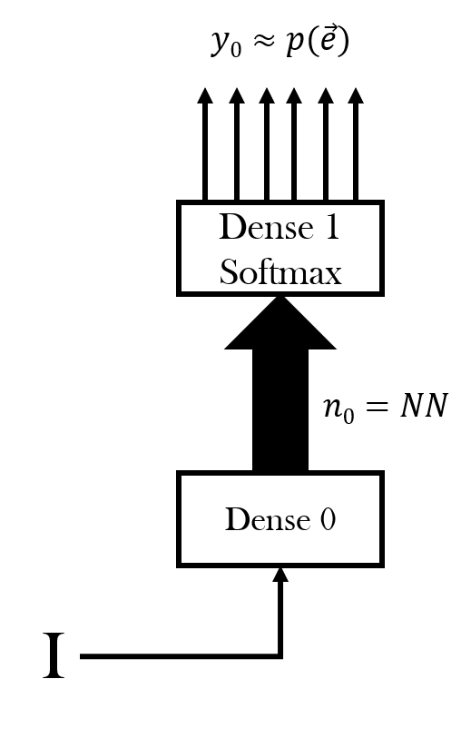
First, we need to see if we have a random variable for emissions in a simple feedforward neural network. In the figure below, every rectangle represents a layer. The lower layer is an ordinary dense layer. The upper layer is also a dense layer whose outputs are in a 1-of-V format where V is the number of vocabulary items, with a softmax function so that the output activations can be interpreted as an emission probability distribution over all possible vocabulary items.
| HMM variable names | RNN Variable Names | |
|
|
|
|
ni | |
|
et | |
|
|
| Generation | Recognition | |
| Input | --------------- | Sequence |
| Output | Random sequence | Score/probability |

| HMM variable names | RNN Variable Names | |
|
|
|
|
ni | |
|
et | 1-hot |
|
|
1-hot |


How do we measure the context captured by our language model? At first glance to the n-gram models you might see that trigram is able to capture more context than bigram models but how can we sure about it? In order to understand if our hypothesis is valid or invalid we need to find a standard way of measuring the error. Here we introduce the perplexity as a way to evaluate your models.
Let's assume that is the input to your model then the perplexity of a sentence W is as below:The success of your model is based on how it performs for test sentences. Lower perplexity for each test sentences means that your model performs better. In real life, it is difficult to achieve but you should try to minimize perplexity per sentence by iterating the experimental steps. Don't forget to report every iteration you did.
We will measure the success of your model by summing up the perplexity of each sentence. The lower total sum will yield higher accuracy. The total perplexity will be calculated as follows:
After you have built one of your proposed models in assignment.cpp, you can run the command make and ./main to compile and run your model. It will print out each test sentence together with your model's output distance for sentence and a total score for your model.
Entropy is the average uncertainty of a random variable. In language, entropy is the information that is produced on the average for each letter of text in the language. It is also known as the average number of bits that we need to encode the information. By definition entropy of a random variable is:
If you look at the definition of the perplexity in Wikipedia, you will see below equation:
Where H(P) is the entropy of the distribution P(X) and X is a random variable over all possible events.
Entropy is the average number of bits to encode the information contained in a random variable. When we have the exponentiation of the entropy it yields to the total amount of all possible information, the weighted average number of choices a random variable has. For example, if the average sentence in the test set could be coded in 100 bits, the model perplexity is 2 100 per sentence.
You need to complete this assignment on CSE Lab2 machines. You don't necessarily need to go to the physical lab in person (although you could). CSE Lab2 has 54 machines, which you can remotely log into with your CSE account. Their hostnames range from csl2wk00.cse.ust.hk to csl2wk53.cse.ust.hk. Create your project under your home directory which is shared among all the CSE Lab2 machines.
For non-CSE students, visit the following link to create your CSE account. https://password.cse.ust.hk:8443/pass.html
In the registration form, there are three "Set the password of" checkboxes. Please check the second and the third checkboxes.
Your home directory in CSE Lab2 has only 100MB disk quota. To see a report of the disk usage in your home directory, you can run du command. It is recommended that you have at least 30MB available before you start this assignment.
Please download the starting pack tarball, and extract it to your home directory on CSE Lab2 machine. This starting pack contains the skeleton code, the feedforward network library and the dataset. The starting pack has the following structure:
assignment1/
├── include/*
├──	lib/*
├──	part_demo/
│   ├── assignment.cpp
|   ├── assignment.hpp
│   ├── main.cpp
│   └── makefile
├──	part_a/
│   ├── report.xlsx    (your report goes here)
│   ├── assignment.cpp (your code goes here)
│   ├── assignment.hpp
│   ├── main.cpp
│   └── makefile
└──	part_b/
    ├── report.xlsx    (your report goes here)
    ├── assignment.cpp (your code goes here)
    ├── assignment.hpp
    ├── main.cpp
    └── makefile
The only two files you need to touch are report.xlsx and assignment.cpp. Please do not touch other files.
After downloading the starting pack, you can run tar -xzvf COMP3211_2019Q1_a2.tgz to extract the starting pack
tar collected all the files into one package, COMP3211_2019Q1_a2.tgz. The command does a couple things:
After you extract the starting pack, go into part_demodirectory and run make and main. These are what you will get:
csl2wk15:skumyol:111> make

      make: Warning: File `main' has modification time 20 s in the future

      make: `main' is up to date.

      make: warning:  Clock skew detected.  Your build may be incomplete.

      csl2wk15:skumyol:112> main

      training

      prediction saved to predict.xml

      total distance: 2779.15
You are provided with a sample RNN architecture in your sample please carefully read the code and provided descriptions. You can take this model as a baseline and compare your outputs with this dummy model.
//
// Created by Dekai WU and YAN Yuchen on 20190424.
//

#include "assignment.hpp"
#include <make_transducer.hpp>
#include <shared_utils.hpp>

using namespace tg;
using namespace std;
namespace part_demo {

    unsigned const NUM_EPOCHS = 4;

    vector<symbol_t> vocab;
    static const unsigned EMBEDDING_SIZE = 32;
    transducer_t embedding_layer;
    transducer_t one_hot;
    transducer_t dense_feedfwd_softmax;
    transducer_t dense_feedfwd_tanh;

    void init(const vector<sentence_t> &training_set) {
      // first you need to assemble the vocab you need
      // in this simple model, the vocab is the top 1000 most frequent tokens in training set
      // we provide a frequent_token_collector utility,
      // that can count token frequencies and collect the top X most frequent tokens
      // all out-of-vocabulary tokens will be treated as "unknown token"
      frequent_token_collector vocab_collector;
      for (const auto &sentence:training_set) {
        for (const auto &token:sentence) {
          vocab_collector.add_occurence(token);
        }
      }
      //Here we are going to define our custom layers that we are going to use in each RNN layer
      //Since each RNN hidden layer is identical we only need to define each layer once.
      //You might see that we are not defining the layers dot_product, -log and sum. Because they are already
      //available in our library and doesn"t reqire a customization
      //since all layers are defined here we can make our rnn by declaring topology over the layers
      vocab = vocab_collector.list_frequent_tokens(1000);
      embedding_layer = make_embedding_lookup(EMBEDDING_SIZE, vocab); //stands for EMB layer in the figure
      one_hot = make_onehot(vocab);  //stands for 1-hot layer in the figure
      dense_feedfwd_softmax = make_dense_feedfwd(vocab.size() + 1, make_log_softmax());// stands for dense 1 log softmax in the figure
      dense_feedfwd_tanh = make_dense_feedfwd(EMBEDDING_SIZE, make_tanh()); // stands for dense 0 tanh
    }

    /**
     * construct an RNN that will evaluate the degree of goodness of a sentence
     * in this demo part, it evaluate the degree of goodness of the first 3 tokens of the sentence
     * \param training_set the set of all training tokens, will be used to construct a vocabulary
     * \return an RNN model
     */
    transducer_t make_rnn_recognizer_3_inputs() {
      auto initial_state = make_const(vector<scalar_t>(EMBEDDING_SIZE, 0));
      auto start_of_sentence = make_const(token_t("<s>"));

      auto cell = compose(make_concatenate(2), dense_feedfwd_tanh);
      auto copy = make_copy(2);

      auto input_pick = make_pick({0, 1, 0, 1, 2});

      auto timestep_0 = compose(group(initial_state, compose(start_of_sentence, embedding_layer)), cell, copy);
      auto timestep_0_to_1 = compose(group(timestep_0, embedding_layer), group(make_identity(), compose(cell, copy)));
      auto timestep_0_to_2 = compose(group(timestep_0_to_1, embedding_layer), group(make_identities(2), cell));

      auto output_pick = make_pick({0, 3, 1, 4, 2, 5});

      auto readout_loss = compose(
              group(compose(dense_feedfwd_softmax, make_tensor_neg()),
                    one_hot), make_dot_product());

      return compose(input_pick, group(timestep_0_to_2, make_identities(3)), output_pick,
                     group(readout_loss, readout_loss, readout_loss), make_tensor_add(3));
    }
}
You already know that in order to construct a feedforward layer, you need to specify the input dimension, output dimension and, activation function. But the sample code indicates a more complex design, now we are going to breakdown the given code into parts. If you read the comments of each layer you might have seen that the layers is shared among time steps therefore, shared by RNN layers as well. Since the logic of customized layers are already explained in code descriptions, we are going to explain the network topology and operations here. It important to mention that time step 0 to 2 is our whole construction and we are going to explain it by breaking it down to time steps. Below is the explanation steps:


In this part, you have to build an RNN to score input sentences with fixed length 4 instead 3.
The first step to scientific research is to observe the data. You are provided with a traindata_length_4.xml and a devdata_length_4.xml for each part of the assignment.
Link to training and test data for you to download:
Traindata: http://hltc.cs.ust.hk/COMP3211_2019Q1_a3/res/traindata_length_4.xml
Devdata: http://hltc.cs.ust.hk/COMP3211_2019Q1_a3/res/devdata_length_4.xml
Both training set and development set are in XML format, in which:
An example of such an xml file is provided here:
<dataset>
    <sent>
        <token>RNNs</token>
        <token>are</token>
        <token>good</token>
        <token>models</token>
    </sent>
</dataset>
You don't need to worry about how to read these XML files into C++ data structure. This dirty part will be handled by our library.
Limiting the sentence size introduces a totally different search space than your previous assignment this dataset is might be more uniform and easier to model using a simple representation such as bigram. But it is not guaranteed, you need to observe data to get an intuition about what kind of language might be required for this task.
Find insightful pattern from the data. The main difference in this part is that, now you have a data with sequences of 4. As you know from previous assignment, you need to observe the to get an insight for your design choice here the sequence limitation is also a part of the effect. Moreover, the distribution of your data is also a fact that you might like to observe where sequence limitation also has an effect. We can give you some hints about how to seek patterns, the number of tokens that the random variable at time step t is a pattern in the data and/or visually inspecting how sparse data is in sequential manner. You better try to answer the question of "what might be the an RNN model's advantages and disadvantages against an n-gram model?" after you see the pattern.
According to the patterns you have observed so far, please propose some your language model. You need to be able to relate your observations in data with your hypothesis. You should be remembering that one of the topic was the bias of the RNN models during the lecture. We strongly suggest for you to have a look at concept of word embeddings thought in the class to understand bias so you can explain your model's bias.
The next step is to compare those models theoretically, in the following aspects:
Write down your proposed hypotheses together with their pros and cons based on questions above.
Here you need to design experiments that validates/invalidates the hypotheses you came up with.
Write a detailed explanation for your each model indicating that how are they reflecting their underlying hypothesis
Write your own C++ codes to define your model.
Build a RNN that reflects your hypothesis. You will be building your own RNN scorers to obtain score for given sentence. Recall that in assignment 2, you designed a feedforward neural network scorer which assigns score for given input. Here, the artificial network you are going to design will take a fixed size of input sequence of length 4. You can think of that your network is a sequence scorer but we still can reach the score of the each token at timestep t. An RNN for handling a fixed sized input is basically a sequence of 4 feedforward neural networks so you can design your neural network accordingly.
When you at the sample code, you can see that the recurrent part is called for each timestep and recurrent part is made of recycled layers. Those recycled layers constitute the hidden layer standing for timesteps 0,1 and 2, in your topology for input size 4 you need to add next timestep as well. So basically, you are going to recycle the same layer used in previous times once more.
Recall that the assignment.cpp, in the starting pack already
contains an RNN to handle first 3 tokens of a sentence:
You can call this RNN as a
transducer which takes some input (based on your design choice) and
gives a score as output. Your model should output a distance given a token
and its context. The distance of a sentence is defined as sum of emissions generated by your RNN model.
In this part, you have to build an RNN to score input sentences having variable length.
The first step to scientific research is to observe the data. You are provided with a traindata.xml and a devdata.xml for each part of the assignment. While part A is consists of sentences of length 4, part B has no restriction over the length of sentences.
Link to training and test data for you to download:
Traindata: http://hltc.cs.ust.hk/COMP3211_2019Q1_a3/res/traindata.xml
Devdata: http://hltc.cs.ust.hk/COMP3211_2019Q1_a3/res/devdata.xml
Both training set and development set are in XML format, in which:
If you look at the below sentence, you see that the bigram and trigram models might fail to understand the relationship between the tokens, for example, you can represent the sequence "every farmer" but can not represent it's relation with "donkey beats it". The information we can obtain from such sequence is indeed has a weak representation due to language bias of the bigram and trigram language models. Therefore, the data itself gives us some ideas about what kind of language bias is necessary in order to create a better model. Now we can talk about the Part A, limiting the sentence length actually reduces the sparsity and the dependencies, consequently, your search space in this part is significantly different than the Part A.
<dataset>
    <sent>
        <token>every</token>
        <token>farmer</token>
        <token>has</token>
        <token>a</token>
        <token>donkey</token>
        <token>beats</token>
        <token>it</token>
    </sent>
</dataset>
You don't need to worry about how to read these XML files into C++ data structure. This dirty part will be handled by our library.
Find insightful pattern from the data. Your data here is same with the previous assignment, you need to observe the to get an insight for your design choice. You need to seek the patterns in way that you get an insight about sequences. Please don't forget that the RNN task indicates long distance dependencies between tokens unlike bigram and trigram models. Thus, you might need to adjust your pattern seeking accordingly.
According to the patterns you have observed so far, please propose some your language model. You need to be able to relate your observations in data with your hypothesis. You should be remembering that one of the topic was the bias of the RNN models during the lecture. We strongly suggest for you to have a look at concept of word embeddings thought in the class to understand bias so you can explain your model's bias.
The next step is to compare those models theoretically, in the following aspects:
Write down your proposed hypotheses together with their pros and cons based on questions above.
Here you need to design experiments that validates/invalidates the hypotheses you came up with.
Write a detailed explanation for your each model indicating that how are they reflecting their underlying hypothesis
Write your own C++ codes to define your model.
Build a RNN that reflects your hypothesis. You will be building your own RNN scorers to obtain score for given sentence. Recall that in assignment 2, you designed a feedforward neural network scorer which assigns score for given input. Here, the artificial network you are going to design will take a dynamic size of input sequence instead of length 4. You can think of that your network is a sequence scorer but we still can reach the score of the each token at timestep t. An RNN for handling a dynamic sized input is basically a sequence of feedforward neural networks of input size.
You have 2 ways to build a recursive network, the first way is hardcoding every possible RNN for different input size which would be challenging to do so another way is using recursion to generate each RNN on the fly. We are going to explain to you how to create recursive RNNs, but First of you need to understand that make_pick, timestep, and readout_loss are subject to recursive part and we will start from input_pick.
2. Timestep layers are actually only one layer (recurrent layer) with recursion except for the first layer for the initial state, thus, we suggest you handle the recursion based on the input size.
timesteps = compose(group(timesteps, embedding_layer), group(make_identities(), compose(cell, copy)));
3. As you saw in the pick diagrams, we need to reorganize the information flow again to provide a valid information to the readout_loss layer. When you go back to sample code, you might see the logic of the output pick, it creates a cross-mapping between two layers. If we'd like to create such a vector on the fly, we need to think about it as a loop again. At each iteration, the iteration counter i should be pushed to the parameter vector of output_pick and i + input_length should also be pushed to the output_pick, in such way each input will be mapped to the exact correspondent identity. i.e input size 3 RNN in the sample code has a mapping of {0, 3, 1, 4, 2, 5} if it we had input size 5 RNN the output pick mappings will be {0, 5, 1, 6, 2, 7, 3, 8, 4, 9}.
4. Readout loss layer input size is always fixed by the output size of the hidden layer, no need for identities as well. So we can group the readout loss layer recursively as input size then use that grouped readout loss layer to compose all structure together. The recursion in the for loop here might look like; layer1 = group(layer1, layer2).
| Graph Representation | Pseudo Code |
 |
A |
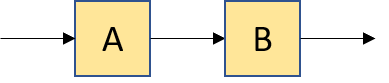 |
compose(A, B) |
 |
compose(A, B, C) // or equivalently compose(compose(A, B), C) |
 |
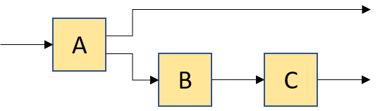
compose(group(A, B), C) |
 |
compose(group(make_identity(), A), B) |
 |
compose(A, group(B, C)) |
 |
compose(make_copy(2), group(A, B)) |
 |
compose(A, group(make_identity(), compose(B, C))) |
 |
compose(A, group(B, C), D) |
In assignment.cpp, it also contains an example on how supply a token together with one/two preceding token as context;
vector<feature_t> get_features(const vector<string> &sentence) {
  // this starting code demonstrate how to trim (or pad) a sentence into length 3

  // if the sentence is shorter than 3 tokens, add some padding at the end to make it length 3
  if(sentence.empty()) {
    return vector<feature_t>{"</s>","</s>","</s>"};
  }
  else if(sentence.size() == 1) {
    return vector<feature_t>{sentence[0],"</s>","</s>"};
  }
  else if(sentence.size() == 2) {
    return vector<feature_t>{sentence[0],sentence[1],"</s>"};
  }

    // if the sentence is longer than 3 tokens, take the first 3 tokens and trash the rest
  else {
    return vector<feature_t>{sentence[0],sentence[1],sentence[2]};
  }
}
In assignment.cpp You need to put your student ID in the global variable STUDENT_ID.
const char* STUDENT_ID = "1900909";
After analyzing why your model went wrong, you should be able to make a better hypothesis. Now you have completed one iteration of scientific research. On the next iteration, you compare your new hypothesis theoretically and empirically again, doing more error analysis, and coming up with more awesome model.
Start another scientific method iteration.
You need to submit a tgz archive named assignment3.tgz via CASS. The tgz archive should ONLY contain two folders as part_a and part_b. Each folder should contain below files.
Due date: 2019 May 12 23:59:00
The initial model that you get from directly modifying the demo code does not count towards a hypothesis. But we assume that the starting code is the hypothesis #1 so you need put the code of your initial model into report.xlsx iteration #1 hypothesis #1 as a record (although they don't count towards your grade). By observing the outcome of the starting code (hypothesis #1), you can form your own hypothesis i.e. hypothesis #2, it is important to denote that you are not required to do error analysis on hypothesis #1. Briefly, your new hypothesis should be based on your observations on the outcome of the previous iteration which you can find it out by running the starting code.
Part A