https://www.oreilly.com/library/view/head-first-data/9780596806224/ch01.html
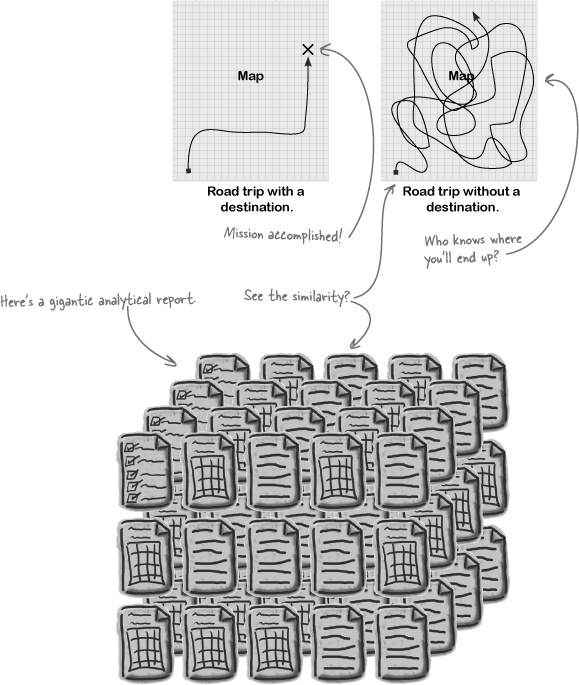
Seek patterns in the data. If you have already begun coding just stop whatever you are doing and read this text. Imagine that you have a map and you want to head a location, first you need to check what path you need to take before heading.

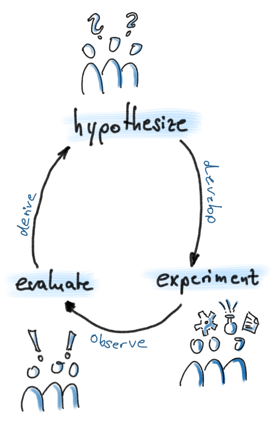
You might think that "I see a bunch of words that don't make sense to me". Just looking at the data itself is not enough to come up with the problems and solutions. The observation phase is all about identifying problems. Let us give you an insight: when you look at the development data, can you see a pattern between the input data and the oracle data? This stage is also called exploratory data analysis. It is a life-saving skill. It will guide you to generate hypotheses that are worthwhile to test.
Generate hypotheses that would explain the pattern. After the previous step you probably have some ideas about what a possible hypothesis might be. In this assignment, your model choices are limited to feedforward neural networks and k nearest neighbors classifiers.
Now you need to hypothesize your own models. You have many options. Generate multiple competing hypotheses; don't just settle for the first option you think of. Some of them might be a good fit to your problem based on your observations. Some of them might not.
Compare and contrast the hypotheses analytically. Now that you have generated a bunch of alternative competing hypotheses, you need to contrast them and discuss their plausibility before testing them. You are already familiar with the terms language bias and search bias. Explain your hypotheses in terms of:
Compare and contrast the hypotheses experimentally.
Do error analysis on the experimental results. What patterns did your hypotheses fail to capture? Why not?
Repeat the scientific method cycle. You have finished one iteration of scientific method. Return to step 2, and generate new hypotheses.
You need to complete this assignment on CSE Lab2 machines. You don't necessarily need to go to the physical lab in person (although you could). CSE Lab2 has 54 machines, which you can remotely log into with your CSE account. Their hostnames range from csl2wk00.cse.ust.hk to csl2wk53.cse.ust.hk. Create your project under your home directory which is shared among all the CSE Lab2 machines.
For non-CSE students, visit the following link to create your CSE account. https://password.cse.ust.hk:8443/pass.html
In the registration form, there are three "Set the password of" checkboxes. Please check the second and the third checkboxes.
Your home directory in CSE Lab2 has only 100MB disk quota. To see a report of the disk usage in your home directory, you can run du command. It is recommended that you have at least 30MB available before you start this assignment.
Please download the starting pack tarball, and extract it to your home directory on CSE Lab2 machine. This starting pack contains the skeleton code, the feedforward network library and the dataset. The starting pack has the following structure:
assignment1/
├── include/
│   └── transducer.hpp
├──	lib/
│   └── transducer.a
└──	src/
    ├── report.xlsx
            (your report goes here)
    ├── assignment.cpp
            (your code goes here)
    ├── traindata.xml
    ├── devdata.xml
    ├── assignment.hpp
	├── main.cpp
    ├── obj/
    └── makefile
The only two files you need to touch are report.xlsx and assignment.cpp. Please do not touch other files.
After downloading the starting pack, you can run tar -xzvf COMP3211_2019Q1_a2.tgz to extract the starting pack
tar collected all the files into one package, COMP3211_2019Q1_a2.tgz. The command does a couple things:
After you extract the starting pack, go into its src directory and run make. This is what you will get:
The first step to scientific research is to observe the data. You are provided with a traindata.xml and a devdata.xml. They represent the training set and the development test set respectively.
Both training set and development set are in XML format, in which:
An example of such an xml file is provided here:
<dataset>
    <sent>
        <token>time</token>
        <token>flies</token>
        <token>like</token>
        <token>an</token>
        <token>arrow</token>
    </sent>
</dataset>
You don't need to worry about how to read these XML files into C++ data structure. This dirty part will be handled by our library.
Find insightful pattern from the data. In the last assignment, most of you just scrolled through the data and concluded something like "the data is from newspaper", which doesn't help you to design model. This time your observations should be insightful so that they will be foundations for your hypotheses and report them accordingly.
Recall that: In the last assignment, we were dealing with English words and as mentioned in class as well, a good observation would be token q is often followed u but never followed by z which might be a foundation of bigram hypothesis . Same goes to english sentences, I is rarely followed by is.
Good observations comes from statistical analysis. For example, here are some directions may be useful in finding patterns.
Report your observations about the data. You might use the hints we gave you but you are not limited with them.
According to the patterns you have observed so far, please propose some language models. The next step is to compare those models theoretically, in the following aspects:
Write down your proposed hypotheses together with their pros and cons based on questions above.
Here you need to design experiments that validates/invalidates the hypotheses you came up with.
Write a detailed explanation for your each model indicating that how are they reflecting their underlying hypothesis
Write your own C++ codes to define your model.
Build a feedforward network that reflects your hypothesis. The assignment.cpp, in the starting pack already contains a fully functioning 2-layer feedforward network as an example:
You will be building your own feedforward network scorers to obtain score for given sentence. Recall that in assignment 1, you had to use Dijkstras' algorithm to find the best output given input and transition scores you obtain from language model. Here, the training component is more transparent and open to your customization so the scores are also depending on your design of model.
As you can see below, you are provided with an assignment.cpp with example code. You can call this feedforward neural network as a transducer which takes 1 or more inputs (based on your design choice) and gives a score as output. Your model should output a distance given a token and its context. The distance of a sentence is defined as sum of distance of its tokens.
/**
/**
 * create your custom classifier by combining transducers
 * the input to your classifier will a list of tokens
 * \param vocab a list of all possible words
 * \param postags a list of all possible POS tags
 * \return
 */
transducer_t your_classifier(const vector<token_t> &vocab) {

  // in this starting code, we demonstrates how to construct a 2-layer feedforward neural network
  // that takes 2 tokens as features

  // embedding lookup layer is mathematically equivalent to
  // a 1-hot layer followed by a dense layer with identity activation
  // but trains faster then composing those two separately
  auto embedding_lookup = make_embedding_lookup(64, vocab);

  // create the first dense feedforward layer,
  // with 64 output units and tanh as activation function
  auto dense0 = make_dense_feedfwd(64, make_tanh());

  // create the final dense feedforward layer
  // since it is the final layer, it need to output the same dimension as the vocabuary
  // actually I lied. the test data may contain tokens that is out of the vocabulary.
  // all those unknown token will become a special UNK token
  // as a result you need vocab size and +1, +1 is for UNK.
  auto dense1 = make_dense_feedfwd(vocab.size()+1, make_softmax());

  auto onehot = make_onehot(vocab);

  auto dot_product = make_dot_product();

  // connect these layers together
  // composing A and B means first apply A, and then take the output of A and feed into B
  return compose(group(compose(embedding_lookup, dense0, dense1), onehot), dot_product);
}
Conceptually, in order to construct a feedforward layer, you need to specify the input dimension, output dimension and activation function. But in the starting pack code, we can see that only the output dimension and activation function is explicitly specified. This is because the layer will eventually know the input dimension by looking at the input it receives anyway.
| Graph Representation | Pseudo Code |
 |
A |
 |
compose(A, B) |
 |
compose(A, B, C) // or equivalently compose(compose(A, B), C) |
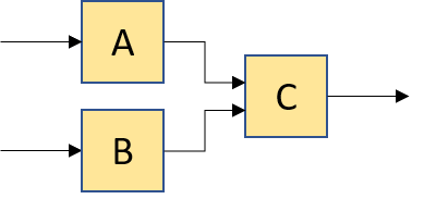 |
compose(group(A, B), C) |
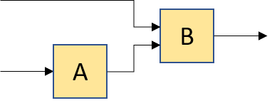 |
compose(group(make_identity(), A), B) |
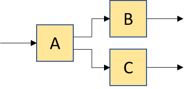 |
compose(A, group(B, C)) |
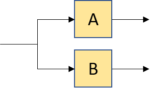 |
compose(make_copy(2), group(A, B)) |
 |
compose(A, group(make_identity(), compose(B, C))) |
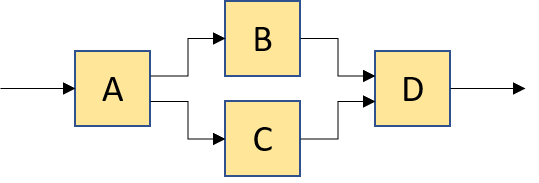 |
compose(A, group(B, C), D) |
In assignment.cpp, it also contains an example on how supply a token together with one/two preceding token as context;
/**
 * Your model requires other tokens as "context" input
 * this function defines the inputs that your model expects
 * \param sentence the sentence that the target token is coming from
 * \param token_index the position of the target token in the sentence
 * \return trigram, bigram or unigram tokens to feed to your model. note that before feeding to your model,
 *         these tokens will be automatically converted into 1-hot representation.
*/
vector <token_t> get_features(const vector <token_t> &sentence, unsigned token_index) {

  // in these starting code, we demonstrate how to feed the target token,
  // together with its preceding token as context.

  if (token_index > 1) {

    // when the target token is not the first token of the sentence, we just need to
    // feed the target token and its previous token to the model
    return vector <token_t> {sentence[token_index], sentence[token_index - 1], sentence[token_index - 2]};
  } else if (token_index > 0) {

    // in case the target token is the first token, we need to invent a dummy previous token.
    // this is because a feedforward network expects consistent input dimensions.
    // if sometimes you give the feedforward network 1 token as input,
    // sometimes you give it 2 tokens as input, then the feedforward network will be angry.

    // there is nothing special about the string "<s>". you can pick whatever you want as long as
    // it doesn't appear in the vocabulary
    return vector <token_t> {sentence[token_index], sentence[token_index - 1], "<s>"};
  } else {

    // in case the target token is the first token, we need to invent a dummy previous token.
    // this is because a feedforward network expects consistent input dimensions.
    // if sometimes you give the feedforward network 1 token as input,
    // sometimes you give it 2 tokens as input, then the feedforward network will be angry.

    // there is nothing special about the string "<s>". you can pick whatever you want as long as
    // it doesn't appear in the vocabulary
    return vector <token_t> {sentence[token_index], "<s>", "<s>"};
  }
}
In assignment.cpp You need to put your student ID in the global variable STUDENT_ID.
const char* STUDENT_ID = "1900909";
How do we measure the context captured by our language model? At first glance to the n-gram models you might see that trigram is able to capture more context than bigram models but how can we sure about it? In order to understand if our hypothesis is valid or invalid we need to find a standard way of measuring the error. Here we introduce the cross-entropy as a way to evaluate your models.
Entropy is the average uncertainty of a random variable. In language, entropy is the information that is produced on the average for each letter of text in the language. It is also known as the average number of bits that we need to encode the information. By definition entropy of a random variable is:
If you look at the definition of the perplexity in Wikipedia, you will see below equation:
Where H(P) is the entropy of the distribution P(X) and X is a random variable over all possible events.
Entropy is the average number of bits to encode the information contained in a random variable. When we have the exponentiation of the entropy it yields to the total amount of all possible information, the weighted average number of choices a random variable has. For example, if the average sentence in the test set could be coded in 100 bits, the model perplexity is 2100 per sentence.
Cross-entropy loss, or log loss, measures the performance of a classification model whose output is a probability value between 0 and 1. Cross-entropy loss increases as the predicted probability diverges from the actual label. So predicting a probability of .012 when the actual observation label is 1 would be bad and result in a high loss value. A perfect model would have a log loss of 0.
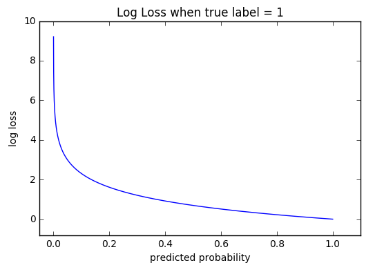
The graph above shows the range of possible loss values given a true observation (isDog = 1). As the predicted probability approaches 1, log loss slowly decreases. As the predicted probability decreases, however, the log loss increases rapidly. Log loss penalizes both types of errors, but especially those predictions that are confident and wrong! Cross-entropy and log loss are slightly different depending on context, but in machine learning when calculating error rates between 0 and 1 they resolve to the same thing. Below you see the formal definition of the binary cross-entropy for a 2-class classification problem where y is a binary variable (0 or 1) indicating that if a predicted token is valid or not and p stands for the probability of the predicted token.
When you run the main you will see a total entropy of your model, lower the total entropy better your model. You will also see a generated file named predicted.xml it will show you the probabilities of each test instance generated by your model and it is for you to understand the behavior of your model. Now you can inspect the outcome of your hypotheses in more detail, wish you an adequate scientific setup.
After analyzing why your model went wrong, you should be able to make a better hypothesis. Now you have completed one iteration of scientific research. On the next iteration, you compare your new hypothesis theoretically and empirically again, doing more error analysis, and coming up with more awesome model.
Start another scientific method iteration.
You need to submit a tgz archive named assignment2.tgz via CASS. The tgz archive should ONLY contain the following two files:
Due date: 2019 April 15 23:59:00